Part II - Deploying Ultralytics YOLO11 to Production Environments
Configuring, deploying and testing YOLO11 with Triton Inference Server. Using Supervision to draw detections on images.
🚨 This is Part II of the “Deploying YOLO11 with Triton” series.
Go to Part I
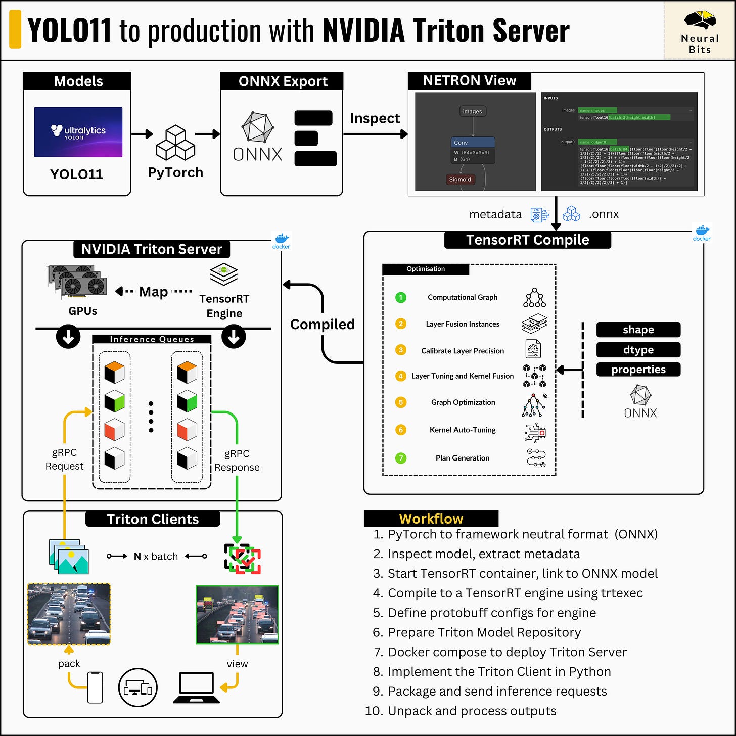
In this article, you will learn to:
Configure the gRPC model API interface
Define the model repository for the NVIDIA Triton Server
Deploy the Triton server using Docker Compose
Implement the TritonClient and submit inference requests
Use Supervision to draw detections
Table of Contents:
NVIDIA Triton Inference Server
Model Protobuf Configs
Implementing the Client
Test the deployment
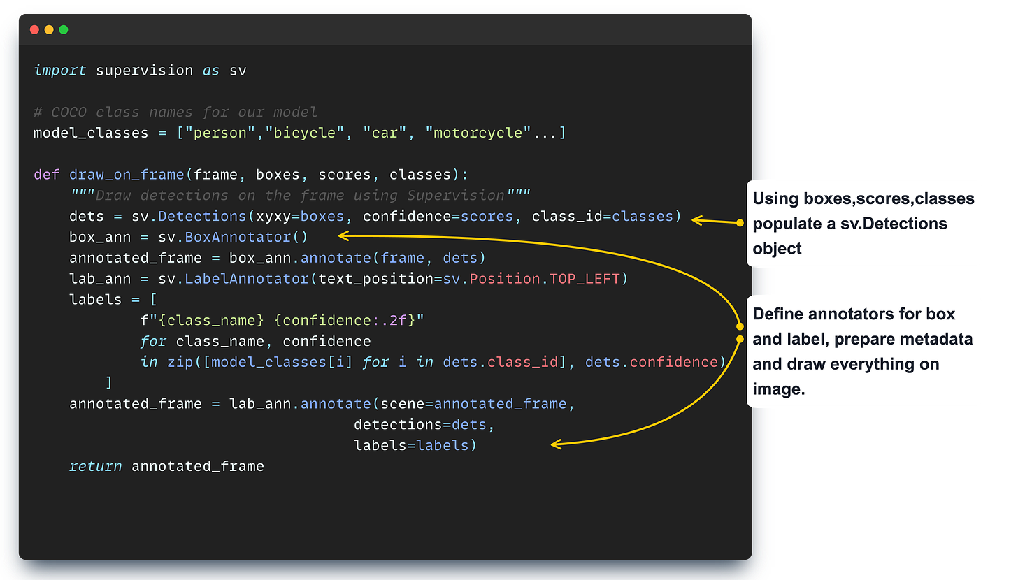
Draw detections using the Roboflow Supervision library
NVIDIA Triton Inference Server
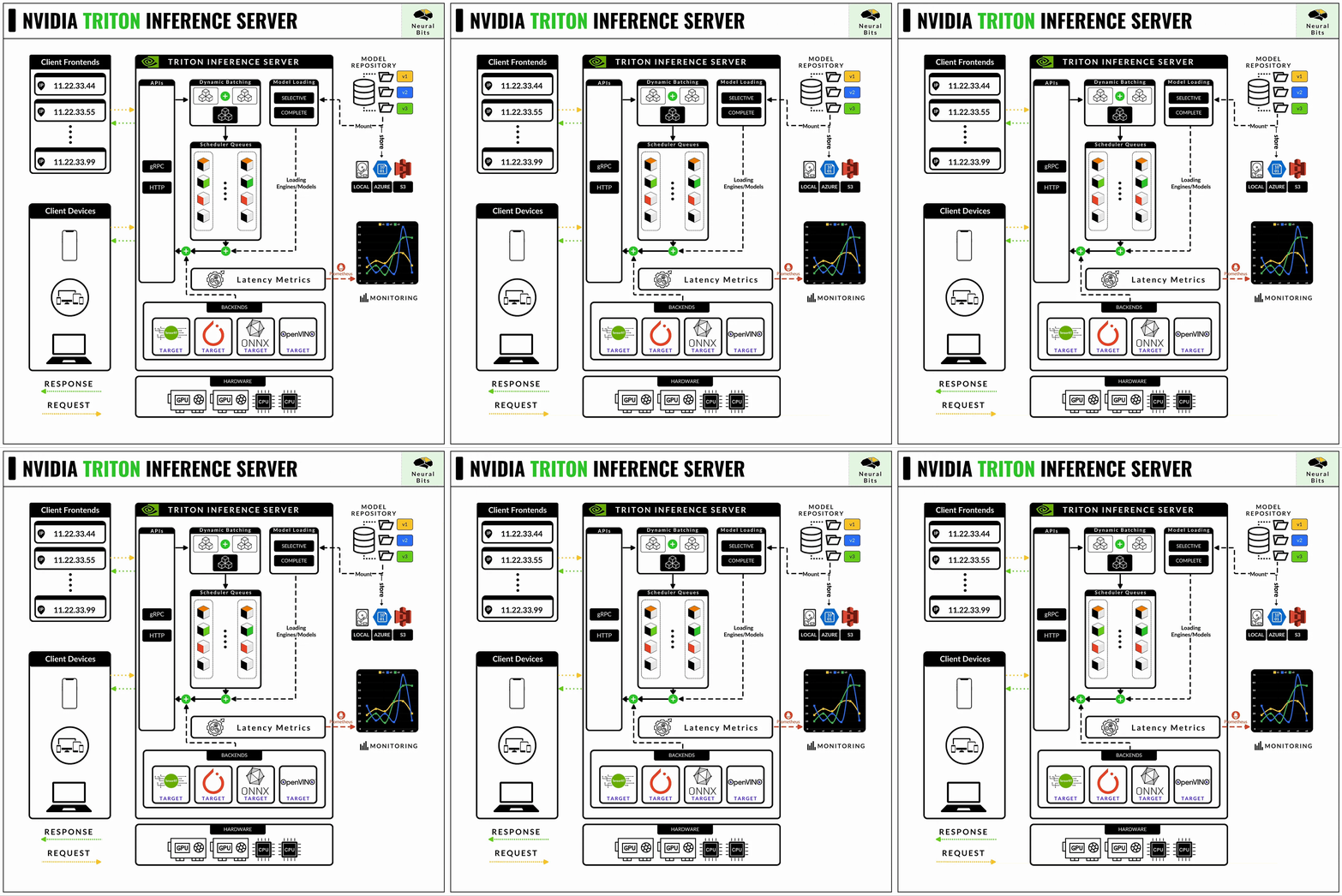
NVIDIA’s Triton Inference Server is currently the most powerful and optimized model-serving framework for any Deep Learning model workload.
📝 See this article, for a complete guide on NVIDIA Triton Server.
The API that defines how Deep Learning models are served in Triton, and how the server should route inference requests is structured via Protobuf config files, attached to each model or pipeline of models.
Let’s see how to define the Protobuf files for our YOLO 11 TensorRT engine.
Model Protobuf Configs
Protocol buffers (protobuf) are Google’s language-neutral, platform-neutral, extensible mechanism for serializing structured data – think XML, but smaller, faster, and simpler.
We define once how the data is structured, then we can use specially generated source code to easily write and read the structured data to and from a variety of data streams and using a variety of languages.
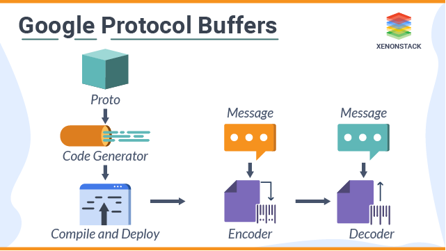
NVIDIA Triton uses Protobuf for two main reasons:
Efficient Data Handling - as it handles large volumes of data in real-time, protobufs allow for a compact way to manage data, helping reduce latency and improve overall performance.
IPC (inter-process communication) - apart from client/server communication, which has to be low-latency, Triton also has to manage internal calls such as dynamic batching, inference scheduling, and queue management—all done through protobuf.
Next, let’s understand what key fields we should specify for our model in Protobuf text format:
The model_name and version so Triton knows how to do the routing.
The platform so Triton knows which ExecutionBackend (e.g. PyTorch, TensorRT, MXNet) to use.
The max_batch_size so Triton knows how to schedule and group inference requests.
The inputs/outputs configurations so Triton knows what shapes and tensor types to expect.
These 4 fields are required in config.pbtxt for a model to be deployable. The list of fields can extend with optional ones, as Triton allows for low-level configuration.
💡 You can think of config.pbtxt + Triton as similar to how Pydantic + FastAPI works. In FastAPI you can specify a custom pydantic model for Response payloads to validate that a client sends that exact object structure for you to deserialize.
Now, each model in Triton has to follow this folder structure:
model_A
  └── 1
      └──model_v1.pt
  └── 2
      └──model_v2.pt
  └── config.pbtxt
💡The term Model Repository refers to a folder that can contain 1 or multiple models structured as showcased above. It is the parent folder for all our models to be deployed with Triton.
Having covered the required theory, let’s get practical and define the actual YOLO 11 model configurations.
Now, here’s how config.pbtxt will look like:
name: "yolov11-engine"
platform: "tensorrt_plan"
max_batch_size: 8

input [
    {
        name: "images"
        data_type: TYPE_FP16
        format: FORMAT_NCHW
        dims: [3, 640, 640]
    }
]

output [
    {
        name: "output0"
        data_type: TYPE_FP16
        dims: [84, 8400]
    }
]
From the previous article, when we compiled the ONNX model with TensorRT, we specified the max_batch_size to be 8, using the maxShapes argument when calling the trtexec command within the TensorRT docker container. For precision, we specified Float16 using the —fp16 argument.
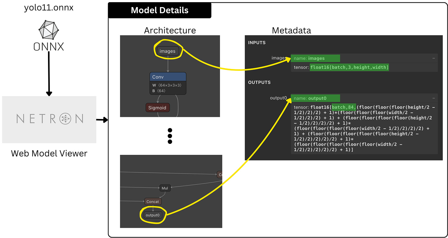
Since we have 1 input layer and 1 output layer, our input-output entries in this config will be lists of length 1. For each layer, we need to specify the name and dimensions (dims), fields that we can get from inspecting the ONNX model using Netron Web Viewer.
Netron is a neural network model visualization tool. It supports models in different formats such as ONNX, TFLite, CoreML and Keras.
After opening the Netron app, we simply load our ONNX model and we’ll see the model architecture on the central panel, and associated metadata on the right.
Now that we have completed the config for the model, we have to create a Triton Model Repository structure and test our deployment.
Triton Model Repository
From the previous article, we’ve already compiled our model into a TensorRT engine and saved it under model.plan, we just moved the file here.
yolov11-engine       # model name, as specified in config
  └── 1             # model version, Triton accepts only INT values
      └──model.plan # our YOLO 11 TensorRT engine
  └── config.pbtxt  # the config written above
Next, let’s organize and move it under a model_repository folder to adhere to Triton’s structure:
mkdir model_repository && mv yolo11-engine model_repository/We’ll set up the Triton Server to test the deployment using a docker-compose.yaml file.
version: '3.4'

services:
  triton_server:
    container_name: triton-inference-server-23.10
    image: nvcr.io/nvidia/tritonserver:23.10-py3
    privileged: true
    ports:
      - 8001:8001
      - 8002:8002
    deploy:
      resources:
        reservations:
          devices:
            - driver: nvidia
              capabilities: [gpu]
    volumes:
      - ${PWD}/model_repository:/models
    command: ["tritonserver", "--model-repository=/models"]
And now, let’s test our deployment by running this command:
docker compose -f docker-compose.yaml upAfter the container starts, we should see this log output, marking a successful deployment.
The server part is done, now we’ll have to implement a client to communicate with the server and test our model deployment.
Implementing the Triton Client
We are going to start by installing the tritonclient python package. Next, let’s connect to the server and test if everything works as expected. Since we’re going to communicate with the server via gRPC, here’s how the implementation looks like:
import cv2
import numpy as np
import tritonclient.grpc as grpcclient
from numpy.typing import NDArray
from tritonclient.utils import (
    np_to_triton_dtype,
)

model_name = "yolov11-engine"
model_vers = "1"

triton_client = grpcclient.InferenceServerClient(
                url="localhost:8001",
                verbose=False)

# Healthcheck (both should be true)
is_live = triton_client.is_server_live()
is_model_ready = triton_client.is_model_ready(model_name, model_vers)
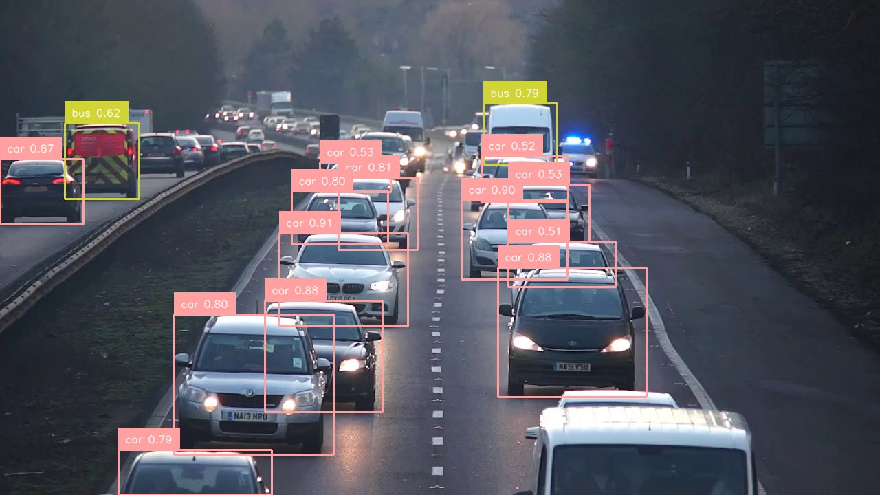
Next, let’s test with an actual image. Here’s the source image we’re going to use:
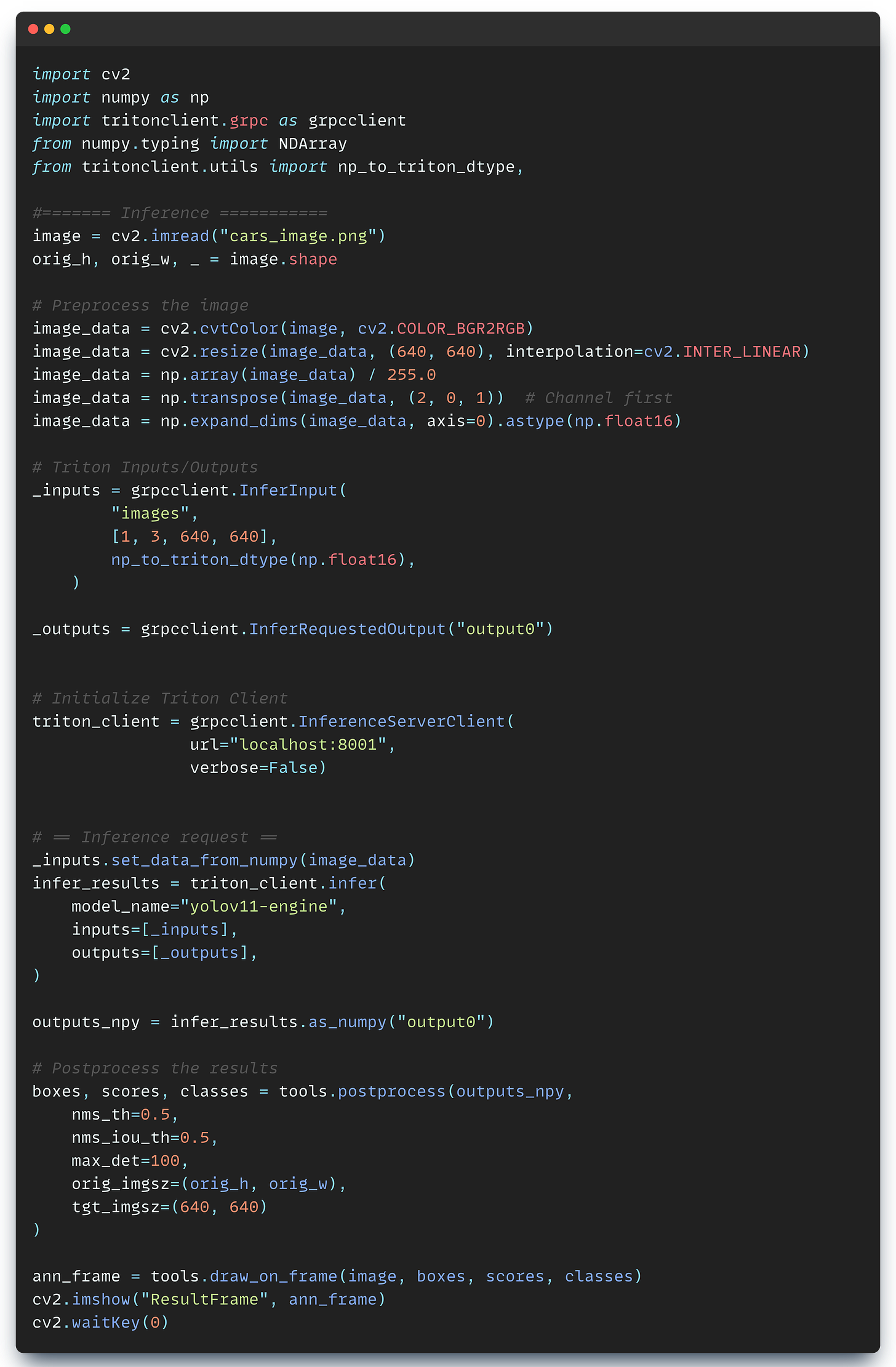
The deployed model expects the input_data in a specific format, as we’ve configured in config.pbtxt with FP16 as precision, and [3, 640, 640] as the input shape.
This preprocessing code transforms the image from its default format of UINT8 data type and (720, 1280, 3) shape as it was loaded by OpenCV (cv2) to the expected format of FLOAT16 data type and (3, 640, 640).
Now, we need to define the gRPC _inputs/outputs_ placeholder objects that will be deserialized by the server, populate, and send an inference request.
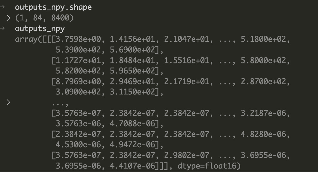
When we inspect the contents of outputs_npy, we’ll get a tensor with the shape we’ve specified in the config.pbtxt (84, 8400) where N = 1 because we had a single image.
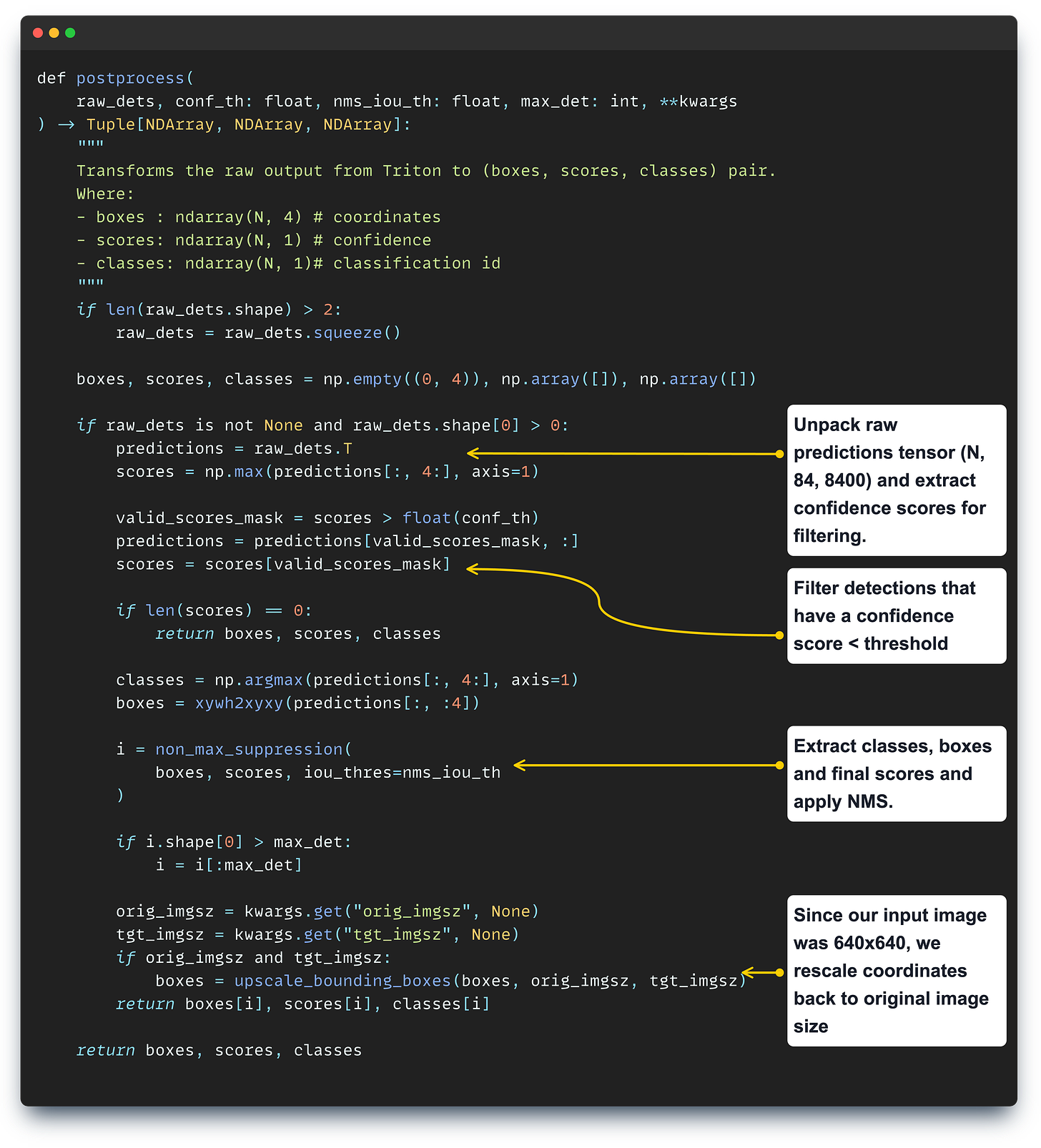
Now, we’ll have to unpack the outputs and extract what we’re interested in which are BoundingBoxes, Classes, and ConfidenceScores.
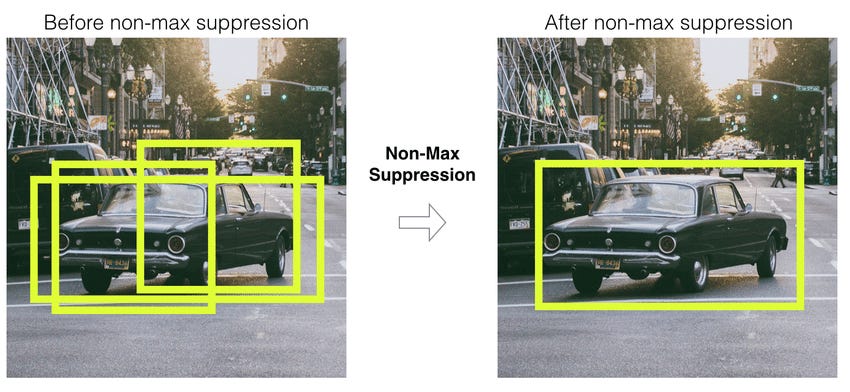
Every model in the YOLO family has a complex post-processing workflow, which involves extracting all bounding boxes, filtering duplicates using the IoU (Intersection over Union) metric, and applying NonMaximumSuppression which filters detected boxes to keep only the relevant instances.
Let’s cover the functionality of the postprocessing step:
After post-processing, once we have formatted boxes, scores, and classes we will use Roboflow’s Supervision to draw detections onto our image.
And lastly, here’s the result, viewing the “annotated_frame” image:
Takeaways
In this article, we’ve completed the deployment of Ultralytics YOLO11 with NVIDIA Triton Inference Server, building an efficient setup for production-ready workloads.
You’ve learned about the process required to optimize and deploy a TensorRT engine with Triton. If you detach and apply these steps to any other model - you could build production-ready inference services using the most efficient model-serving framework.
The complete code for the entire series will soon be uploaded on Neural Bits Github, make sure to follow and star the repo.
Stay tuned, see you next week! 🤗
→ If not specified, all images used are created by the author.


