Part I - Deploying Ultralytics YOLO11 to Production Environments

Learn to optimize YOLO11 (SOTA model for Object Detection) using NVIDIA TensorRT Compiler in a step-by-step walkthrough.

Oct 29, 2024

🚨 This is Part I of the “Deploying YOLO11 with Triton” series.

Go to Part II

In this article, you will learn:

What is YOLO, downloading and preparing the environment
What is ONNX and how to export YOLO 11 to ONNX format
How to define and update an OmegaConf configuration
How to compile the YOLO11 ONNX model using NVIDIA’s TensorRT Compiler

Last month, Ultralytics released the latest model from the YOLO (You Only Look Once), model family, coined as YOLO 11 which comes as a successor to the previous YOLOv10 model from Ultralytics.

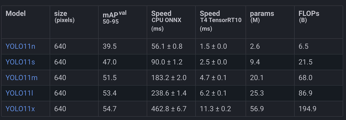
From the benchmarks, YOLO 11 achieves ~2% higher mAP while shaving off up to 22% of the model size.

📌 The mAP (mean Average Precision) is a metric used to measure the performance of an object detection model. It consists of 4 other sub metrics for this task: Confusion Matrix, Intersection over Union, Precision and Recall.

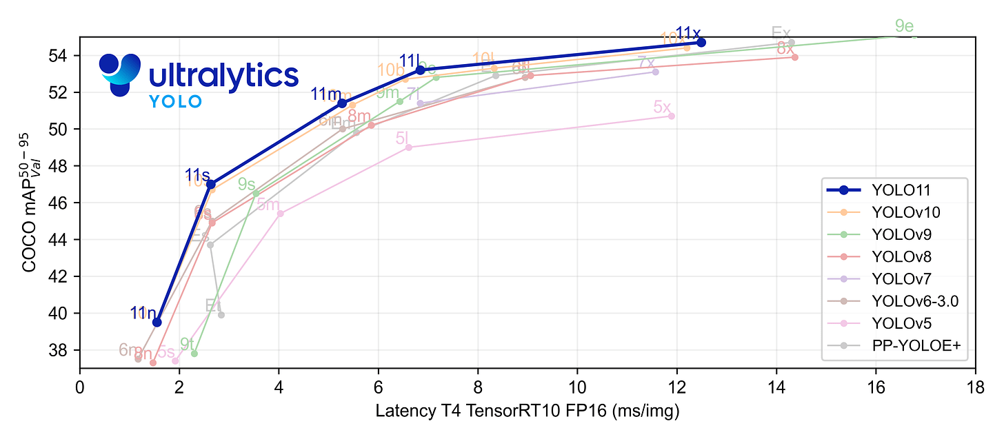
YOLO11 Performance Plots — Image from Source

Although the YOLO model family is a powerful suite of models applied to vision tasks, there’s still a lack of resources that show, 0 to 100, how to deploy them in a compute-efficient production scenario.

In this 2-article series, we’ll cover that process in an end-to-end manner, where you’ll be able to execute and code along each step, to prepare your model for a production deployment using the most advanced model serving framework, NVIDIA Triton Inference Server.

About YOLO

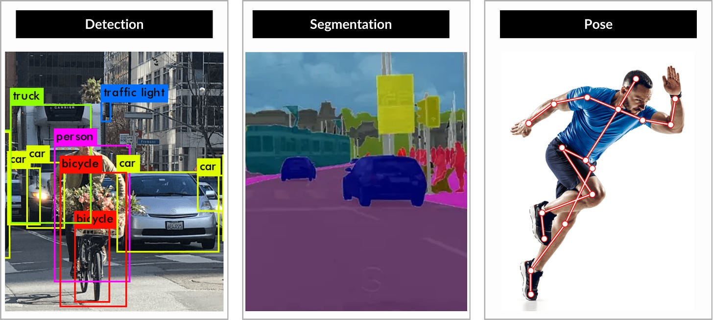
YOLO models are the most popular choice for real-time Deep Learning on Vision Tasks, with tasks spanning across:

Detection - detecting objects in images/videos, drawing a bounding box around them
Segmentation - delimiting objects and instances with pixel accuracy, such as body organs in a CT scan.
Pose - tracking key points, such as human body joints.

YOLO is a single-stage detector, handling both object identification and classification in a single pass of the network. In two-stage models, one model would be used to extract regions of objects, and a second model to classify and further refine the localization. (FastRCNN)

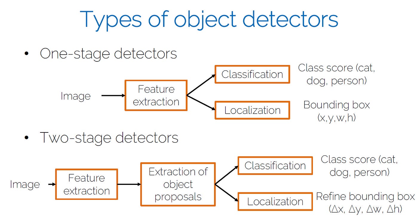
As an image goes through the network, it will follow this process:

Backbone - extracting essential features using multiple Convolution layers.
Neck - Merging feature maps across multiple scales.
Head - generate predictions:
1. Bounding Box coordinates
2. Class scores: for each class, [0.0 - 1.0] confidence score of object belonging to that class
3. Objectness score: probability score that an object is inside the bounding box

The model outputs will be a raw tensor from which we’ll extract these results.

In the next section, we’ll install Ultralytics, download a YOLO 11 checkpoint, and convert it to ONNX format.

What is ONNX

📌 The ONNX acronym comes from Open-Neural-Network-Exchange and it refers to an open format built to represent machine learning models.

ONNX defines a common set of operators that are the building blocks of any Deep Learning model - and a common file format to enable AI developers to use models with a variety of frameworks, tools, runtimes, and compilers.

A model in ONNX format could be parsed and loaded in multiple frameworks, be it PyTorch, TensorFlow, CoreML, or HuggingFace’s Optimum.

ⓘ For a more in-depth on TensorRT, ONNX and PyTorch inference engines, see this detailed article → 3 Inference Engines

Exporting YOLO11 to ONNX

Before starting and verifying the export, we must first prepare the environment.

For that, we’ll install the required Python packages, and define a .yaml configuration file with our model export parameters so that we won’t have to hardcode arguments and load it using OmegaConf.

📌 OmegaConf is a hierarchical configuration system in Python, which allows developers to manipulate multiple config files without manual interventions. Across ML/AI projects, it’s one of the best tools to handle and manage config files.

Let’s install the required packages:

pip install ultralytics, omegaconf, docker

Next, we would have to download a YOLO11.pt pre-trained model. Let’s pick the m-medium version (20.1M params), trained on the COCO dataset.

wget https://github.com/ultralytics/assets/releases/download/v8.3.0/yolo11m.pt

Now, let’s define the configuration file, and call it export.yaml

onnx:
  weights_path: yolov11m.pt
  is_half: false                # export the model in FP16 format
  is_dynamic: true              # the .onnx model has dynamic batch size
  is_simplified: true           # will optimize layers to reduce size
  with_nms: true                # add NonMaximumSuppresion head
  image_size: 640               # the input layer shape (Nx3x640x640)
  device: cuda:0                # device used for export

📌 A dynamic batch size means that the ONNX model will not enforce any batch size, being exported in a configurable state. We’ll then further control the batch size when compiling to TensorRT.

We’ll use OmegaConf to load and parse this config file and with the parameters extracted, we’ll call the ONNX export method.

import os
import ultralytics as ul
from omegaconf import OmegaConf, DictConfig

export_config_path = "export.yaml"
export_cfg = OmegaConf.load(export_config_path)

onnx_cfg = export_cfg.get("onnx")

model = ul.YOLO(model=onnx_cfg["weights_path"])
onnx_path = model.export(
        format="onnx",
        device=onnx_cfg["device"],
        imgsz=onnx_cfg["image_size"],
        nms=onnx_cfg["with_nms"],
        half=onnx_cfg["is_half"],
        simplify=onnx_cfg["is_simplified"],
        dynamic=onnx_cfg["is_dynamic"]
)

# Update Export Config with ONNX model path
onnx_updated = OmegaConf.merge(
        onnx_cfg,
        DictConfig({"onnx_path": m_path}),
    )
merged = OmegaConf.merge(
        conf,
        DictConfig({"onnx": onnx_updated}),
    )
OmegaConf.save(merged, export_config_path)

After we execute this code block, we’ll get the .onnx model saved on disk in the same root directory as the current script. Apart from the initial parameters, we’ll see an extra one added, the onnx_path which will show where the generated ONNX model was saved.

Next, we’ll use the docker package to spin up a TensorRT container and submit a trtexec compile command for our ONNX model directly from Python, without manually controlling Docker from the terminal.

Compiling ONNX using NVIDIA TensorRT Compiler

Following the same structure, where we keep all our parameters in a configuration file, let’s append the parameters for our ONNX → TensorRT process, in our export.yaml config file.

onnx:
    .... (as before)

tensorrt:
  device: 0
  minShapes: images:1x3x640x640   # images is the Input Layer name
  optShapes: images:4x3x640x640   # 1,4,8 are the preferred batch sizes
  maxShapes: images:8x3x640x640   # 3x640x640 represents the Input Shape
  dtype: fp16
  image: nvcr.io/nvidia/tensorrt:22.08-py3

Here, we have specified that:

We’ll use GPU device ad idx 0 for compilation
Our TensorRT engine has a dynamic batch shape, with imposed limits of 1 up to 8 images per batch.
Our TensorRT engine will have FP16 precision
We’ll use TensorRT:22.08 Docker Image

📌 The min/opt/max Shapes can be either selected arbitrarly or following a hardware profilling benchmark. These limits specify our preference of batch sizes for inference when we’ll deploy the TensorRT engine with Triton Server.
We’ll get into more details on this aspect in Part II of this article series.

Now, let’s implement the workflow in Python, assemble the docker steps, and trigger the compilation process.

We’ll start by parsing the config

from omegaconf import OmegaConf

export_config_path = "export.yaml"
export_cfg = OmegaConf.load(export_config_path)

onnx_cfg = export_cfg.get("onnx")
trt_cfg = export_cfg.get("tensorrt")

if not onnx_cfg or not trt_cfg:
    raise ValueError(
      "ONNX or TensorRT configuration is missing. Check export.yaml"
    )

Next, we’ll prepare the Docker Environment

import docker

# Ensure GPU access
gpu_devices = [trt_cfg["device"]]
gpu_config = {
  "device_requests": [{"count": len(gpu_devices), "capabilities": [["gpu"]]}],
   "devices": [f"/dev/nvidia{n}" for n in gpu_devices],
}


# Allow container to access the current folder
volume_mapping = {
  f"{Path().resolve()}": {"bind": "/workspace", "mode": "rw"}
}

# Set-up the client
client = docker.from_env()

Here, we’ve specified the GPU configuration such that the Docker Engine can access and use it. If you have a machine with multiple GPUs, you can select a different ID.

Start the Container in Detached Mode

try:
   container = client.containers.run(
        trt_cfg["image"],
        command='sh -c "while true; do sleep 3600; done"',
        detach=True,
        stdout=True,
        stderr=True,
        remove=True,
        volumes=volume_mapping,
        **gpu_config,
        name="onnx2tensorrt-container",
  )

  print("Container started...")

except docker.errors.DockerException as e:
  print(f"Failed to start container: {e}")

Prepare and execute the compile command

try:
  _exec = "trtexec"
  _onnx_path = Path(onnx_cfg["onnx_path"]).stem

  _o2t = f" --onnx=/workspace/{_onnx_path}.onnx --saveEngine=/workspace/model.plan --{trt_cfg['dtype'].lower()}"

  _shapes = f" --minShapes={trt_cfg['minShapes']} --optShapes={trt_cfg['optShapes']} --maxShapes={trt_cfg['maxShapes']}"

  _force_fp16 = f" --fp16 --inputIOFormats=fp16:chw --outputIOFormats=fp16:chw"
  
  command = _exec + _o2t + _shapes + _force_fp16
  exec_result = container.exec_run(command, detach=False)

  if exec_result.exit_code != 0:
    raise RuntimeError(f"Error during conversion: {exec_result.output.decode('utf-8')}")
  else:
    print("Conversion successful.")
    print(exec_result.output.decode("utf-8"))

except Exception as e:
  print(f"Error executing TensorRT conversion command: {e}")
  raise RuntimeError(f"Error executing TensorRT conversion : {e}")

Here, we’ve used trtexec and the following parameters:

—onnx - path to the ONNX model
—saveEngine - where to save the compiled TensorRT engine
—min/opt/maxShapes - to specify the dynamic batch preferences
—fp16 - to specify the Float16 precision of our TensorRT engine
—inputIOFormats - to specify input layer mapping to chw (channels, height, width)
—outputIOFormats - same as above, for the output layers

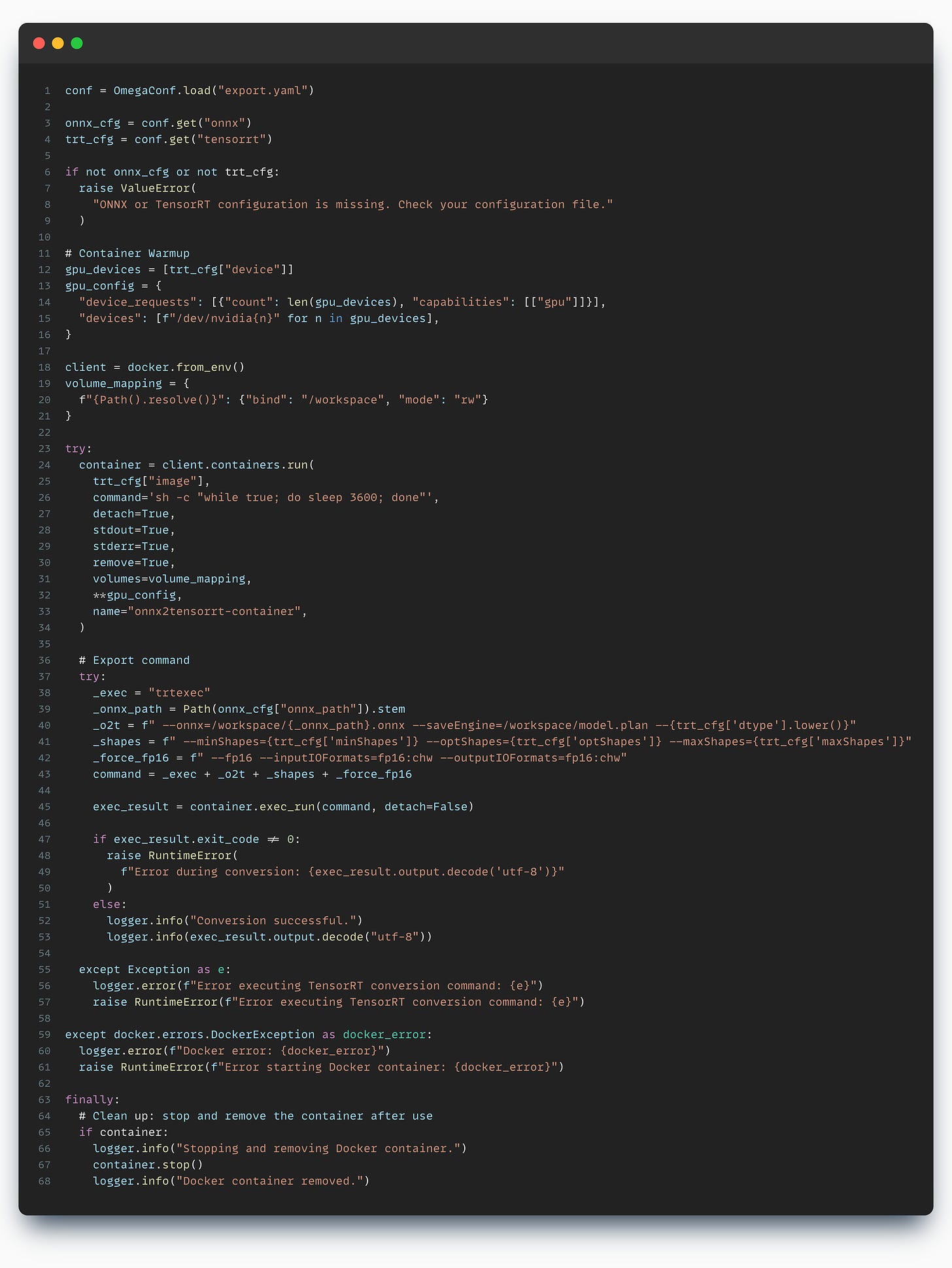
Finally, we’ve concatenated the entire command and started the compilation. The entire code script would look like this:

The output we’ll see after the compilation is done will describe the profiling report for our TensorRT engine on the GPU model we’ve compiled it on.

📌 A TensorRT engine is closely linked to the GPU it was compiled on, because during compilation the model graph is partitioned in such a way that is optimal for that specific GPU architecture.
For instance, if we compile a model on a NVIDIA RTX3080 - it would not work on a NVIDIA V100, due to different chip architectures.

Here’s how the output logs would look like:

[10/04/2024-13:24:14] [I] === Performance summary ===
[10/04/2024-13:24:14] [I] Throughput: 284.831 qps

[10/04/2024-13:24:14] [I] Latency: min = 4.74451 ms, max = 4.80347 ms, mean = 4.77315 ms, median = 4.77563 ms, percentile(90%) = 4.78326 ms, percentile(95%) = 4.78497 ms, percentile(99%) = 4.78979 ms

[10/04/2024-13:24:14] [I] Enqueue Time: min = 0.36731 ms, max = 2.04456 ms, mean = 1.52961 ms, median = 1.54382 ms, percentile(90%) = 1.66931 ms, percentile(95%) = 1.69812 ms, percentile(99%) = 1.96143 ms

[10/04/2024-13:24:14] [I] H2D Latency: min = 0.815796 ms, max = 0.853149 ms, mean = 0.828853 ms, median = 0.830566 ms, percentile(90%) = 0.834229 ms, percentile(95%) = 0.835449 ms, percentile(99%) = 0.846924 ms

[10/04/2024-13:24:14] [I] GPU Compute Time: min = 3.48779 ms, max = 3.51733 ms, mean = 3.50529 ms, median = 3.50818 ms, percentile(90%) = 3.51221 ms, percentile(95%) = 3.51245 ms, percentile(99%) = 3.51538 ms

[10/04/2024-13:24:14] [I] D2H Latency: min = 0.431396 ms, max = 0.442871 ms, mean = 0.439004 ms, median = 0.438965 ms, percentile(90%) = 0.44043 ms, percentile(95%) = 0.440704 ms, percentile(99%) = 0.44165 ms

[10/04/2024-13:24:14] [I] Total Host Walltime: 3.0088 s
[10/04/2024-13:24:14] [I] Total GPU Compute Time: 3.00404 s

This describes the QPS, which shows how many inference requests/s this model can handle on this GPU and other verbose Latency metrics such as :

H2D - (host to device) - which shows how long it takes for the Input tensor to be moved from CPU to GPU.
D2H - (device to host) - the time it takes to move output tensor data from GPU to CPU.

Takeaways

In this article, we’ve covered the first 2 key steps from our process to deploy YOLO 11 in a production-ready setup using NVIDIA Triton Inference Server.

In this example, we’ve showcased how to export a YOLO 11 model to TensorRT format which is optimal for production-ready deployments on NVIDIA GPUs.

This process can be applied to any Deep Learning model architecture.

In Part II of this series, we’ll take the TensorRT compiled engine and adapt it to be deployable with the NVIDIA Triton Inference Server.

Stay tuned, see you next week!

→ If not specified, all images used are created by the author.