3 Inference Engines for optimal throughput
Learn how to speed-up inference using model optimization plans such as Torch.Compile(), ONNXRuntime and TensorRT
Abstract
When deploying machine learning models in production, inference speed is one of the most critical factors to consider.
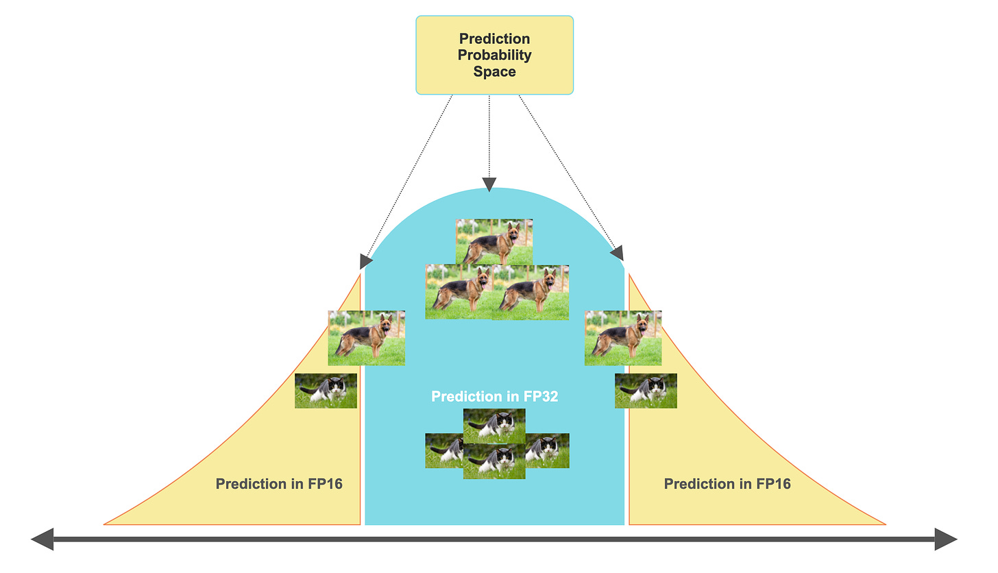
One key aspect influencing inference speed is precision. In a research setting, models are often trained with high precision, such as full FP32 or AMP (Automatic Mixed Precision), where AMP combines FP32 with lower precisions like FP16, allowing some layers to benefit from FP32 calculations while others operate effectively with lower precisions FP16.
Lowering precision reduces the memory footprint required to load a model, as weights are stored in smaller formats. Additionally, it speeds up the forward pass because calculations are done with lower precision.
Doing that, we cut off some of the accuracy, which is expected but the tradeoff is understood in this case as one would rather get a few FP (false positives) than pay/wait more.
However, simply reducing FP32 to FP16 precision isn’t enough to fully optimize a model for deployment, as many other specific techniques could be applied
In this article, we’ll go over 4 pathways of optimizing a model for inference, using a hands-on approach with code as we’ll explore and compare inference speeds:
Default PyTorch
PyTorch Compiled (v2.0+)
ONNX Runtime
NVIDIA TensorRT.
We’ll pick and implement a widely known CNN from scratch - MobileNet v2, optimize and benchmark it across N runs, and then plot the results, explaining what happens under the hood with each optimization technique we use.
Before starting, the code for the entire analysis can be found in Inference Engines Repository [1]
Table of Contents:
1. MobileNetv2 Model Definition
2. Visualizing with GraphViz
3. Benchmark PyTorch & PyTorch Compiled
4. Benchmark ONNXRuntime
5. Benchmark TensorRT Engine
6. Conclusion
Model Definition
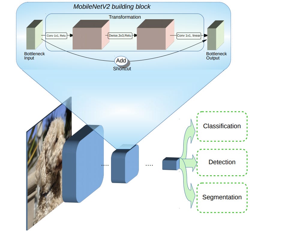
We’ll be using MobileNetV2 which is an efficient deep-learning model architecture designed specifically for mobile and embedded vision applications.
Released in 2019, it builds on top of MobileNetV1 and introduces inverted residuals, linear bottlenecks, and depthwise separable convolutions, which helps it strike a balance between efficiency and performance.
For more details on the model architecture, see MobileNet v2 Google Research Report [4]
Here are the key concepts it introduces:
Inverted Residuals: traditional models, usually expand data before processing, MobileNetV2 first compresses the data, processes it, and then expands it again.
Linear Bottlenecks: in the compression phase, it uses linear layers, where each neuron from the layer before links data to the next layer in a many-to-many relationship - and no information context is lost.
Depthwise Separable Convolutions: it splits the usual convolution process into two simpler steps. First, it processes each color channel of the image separately and then merges them.
Visualizing Model Graph with TorchViz
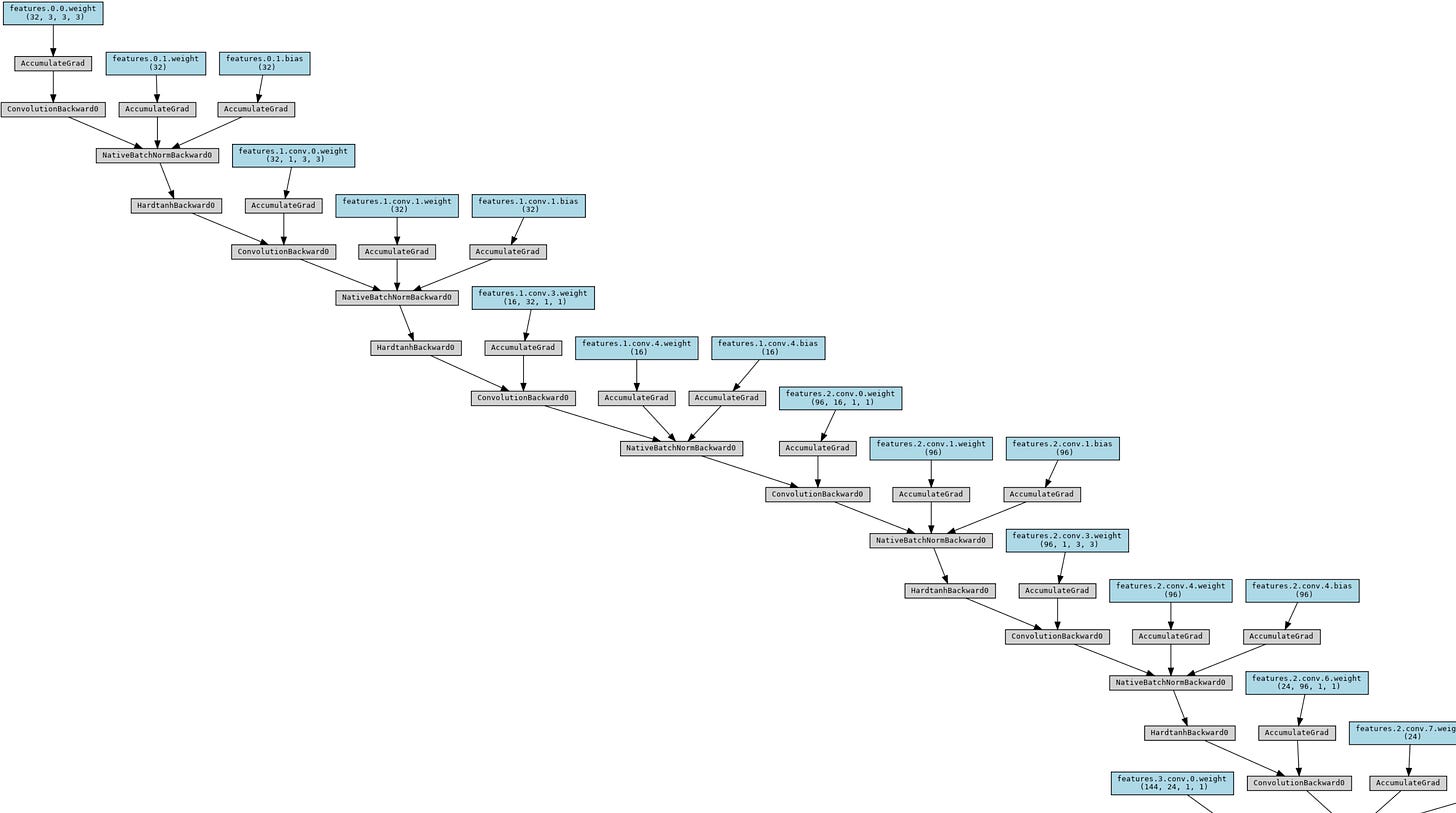
Torchviz [3] is a package to create visualizations of neural networks that are defined as PyTorch modules. It builds on top of GraphViz and renders the network graph and traces.
In our case, we’ve defined our MobileNet v2 model as a PyTorch nn.Module, and then we can visualize it using this code block:
import torch
from torchviz import make_dot
from torch.autograd import Variable

model = MobileNetV2(n_class=2, input_size=224, width_mult=1.)
dummy_input = Variable(torch.randn(1, 3, 224, 224))

# Records the graph of operations
y = model(dummy_input)

# Renders recorded graph
model_graph = make_dot(y, params=dict(model.named_parameters()))

# Saving the graph as an .png image
model_graph.format = 'png'
model_graph.render('mobilenetv2')
model_graph.attr(size='8,6')

from IPython.display import Image
display(Image('mobilenetv2.png'))
Upon executing this block, we’ll get the following visualization (e.g. the start segment of the model graph).
Benchmark PyTorch & PyTorch Compiled
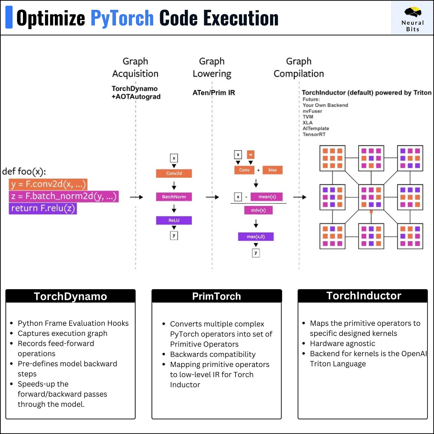
By default, when using the raw PyTorch format for inference, the model execution is in `eager-mode` which means that operations are executed immediately as they are called, which allows for flexibility but impacts performance.
Torch.compile() was introduced starting with PyTorch 2.0+. In a nutshell, torch.compile optimizes the PyTorch code to run faster by JIT (Just In Time)-compiling it into optimized kernels.
Under the hood of torch.compile(), we have these 4 pillars:
𝗧𝗼𝗿𝗰𝗵𝗗𝘆𝗻𝗮𝗺𝗼 - which captures PyTorch programs safely using Python Frame Evaluation Hooks.
𝗔𝗢𝗧𝗔𝘂𝘁𝗼𝗴𝗿𝗮𝗱 - which stands for ahead-of-time autograd overloads PyTorch’s autograd engine to generate ahead-of-time traces through the model
𝗣𝗿𝗶𝗺𝗧𝗼𝗿𝗰𝗵 - a collection of 2000+ PyTorch operators into 250 primitive operators that can be adapted and customized.
𝗧𝗼𝗿𝗰𝗵𝗜𝗻𝗱𝘂𝗰𝘁𝗼𝗿 - the deep learning compiler that generates fast code for multiple accelerators and backends.
Think of TorchInductor as how Java Compiler turns Java code into bytecode that is executed in JVM.
In the same way, TorchInductor compiles PyTorch code into Low-Level IR (intermediate representation code) and then it ports this code to kernels specifically designed for the target architecture (CPUs, TPUs, GPUs, etc.)
Profiling Default vs Compiled versions across 100 runs we’ll get a chart similar to this:
Benchmark ONNX Runtime
ONNX stands for (open-neural-network-exchange) and is an open-source standard for representing deep learning models. An ONNX model is a serialized file containing the computation graph, architecture, weights, and other parameters.
One key detail when exporting models to the ONNX format, is the operator_set version, which helps to ensure portability and reproducibility of the exported models.
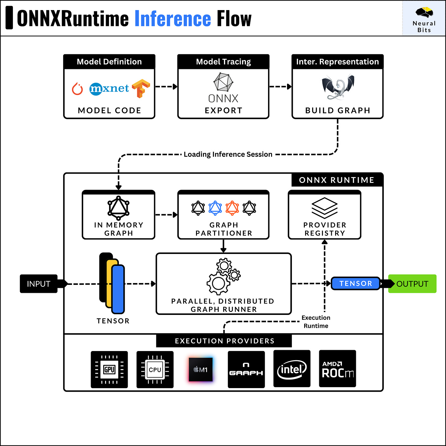
On the other hand, ONNX Runtime [2] is a high-performance runtime engine for executing ONNX models. It was developed by Microsoft to run ONNX models efficiently across different hardware platforms.
An ONNX Runtime [2] inference session loads the model graph, decodes the operator set and trace, and partitions the graph of operations based on the Execution Provider (e.g CPU, CUDA, AMD ROCm) see the flow in the image below.
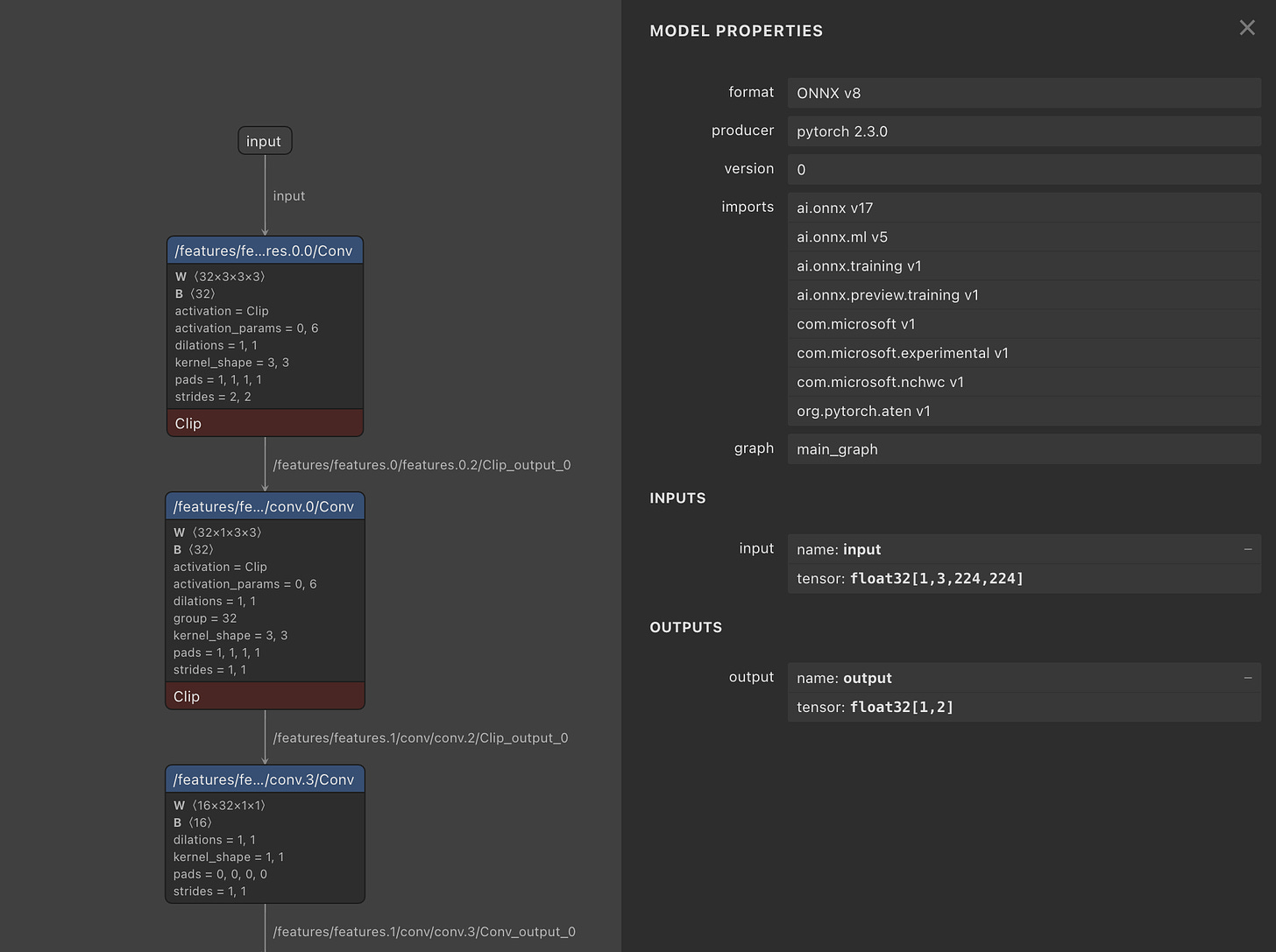
Bonus: ONNX models can be visualized using Netron, for a verbose overview.
Now, if we profile PyTorch vs PyTorch Compiled vs ONNXRuntime across 100 runs we’ll get a chart similar to this one:
To note here that we’ve used the default optimization routine on ONNXRuntime, a more efficient one would imply setting graph_optimization_level and intra_op/inter_op threads specifically.
intra_op - parallelize operations within a single operator
inter_op - parallelize operations across independent operators
Benchmark TensorRT Engine
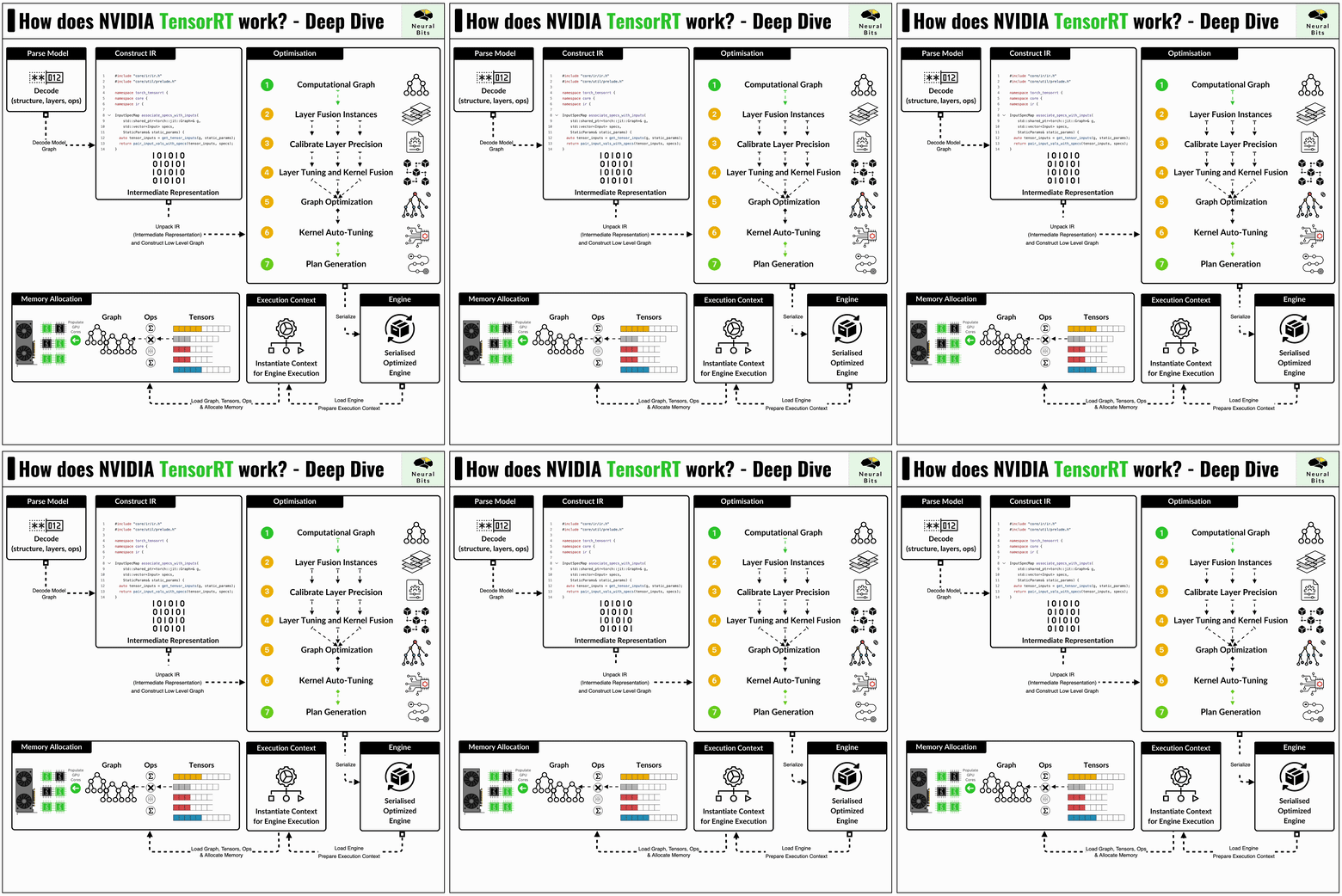
TensorRT format is the lowest level of optimization being the most advanced one in this benchmark set. The TensorRT compiler is specifically designed to maximize performance on NVIDIA GPUs, benefitting from close integration with the underlying CUDA kernels or cuDNN routines for example.
In short, TensorRT applies a series of optimizations, let’s iterate a few ones:
Kernel Fusion - distinct kernels can be fused and calculated on a single data flow. For example, we can fuse a convolution kernel followed by ReLU, and compute the results on a single pass through the data.
Kernel Auto-Tuning - CUDA programming is based on Threads and Blocks, and kernel auto-tuning detects the optimal n_of_threads and n_of_blocks for the specific GPU Architecture, based on its CUDA Cores and Tensor Cores counts.
The most common way to get a model to TensorRT Engine format, is to have it serialized to the ONNX first.
If in the rest of the use-cases we were able to execute the entire workflows using the Poetry env, for TensorRT we’ll use the recommended workflow via docker. The first step is to consult the NVIDIA Compatibility Matrix [3] and select any Container Version that comes with PyTorch 2.0. For this test, we’ll use TensorRT-23.03.
To streamline this process, we’ll execute the workflows using docker-python.
import os
import docker

client = docker.from_env()
container_image = "nvcr.io/nvidia/tensorrt:23.03-py3"
client.images.pull(container_image)

container = client.containers.run(
    container_image,
    detach=True,
    volumes={
        f"{os.getcwd()}/core": {
            "bind": "/workspace",
            "mode": "rw",
        }
    },
    tty=True,
    device_requests=[docker.types.DeviceRequest(count=-1, capabilities=[['gpu']])]
)
In this code, we start the container with GPU access and bind the host path to the container. In the following block, we optimize and serialize the .onnx format into .engine using trtexec.
try:
    code, output = container.exec_run(
        cmd="trtexec --onnx=/workspace/mobilenetv2.onnx --saveEngine=/workspace/mobilenetv2.engine",
        tty=True,
    )

finally:
    container.stop()
    container.remove()
One key detail to mention about TensorRT inference is the low-level memory management, such that we have to allocate memory and manage the H2D (CPU to GPU) and D2H (GPU to CPU) data transfers.
Here’s a glimpse of this low-level setup, where we define and allocate required memory regions for inputs/outputs of our TensorRT Graph.
stream = cuda.Stream()

for binding in self.engine:
  size = (trt.volume(self.engine.get_binding_shape(binding)) * self.max_batch_size)

  host_mem = cuda.pagelocked_empty(size, self.dtype)
  device_mem = cuda.mem_alloc(host_mem.nbytes)
  bindings.append(int(device_mem))

  if self.engine.binding_is_input(binding):
    inputs.append(HostDeviceMem(host_mem, device_mem))
  else:
    outputs.append(HostDeviceMem(host_mem, device_mem))
To profile the TensorRT engine execution, we’ve implemented a custom Python script that we’ll run inside the container, which will measure and report inference times into a .txt file, that we’ll unpack and process later.
Profiling the TensorRT engine over 100 runs, we’ll get this chart:
Conclusion
The full code for this tutorial can be found at Inference Engines Repository [1]
In this article, we’ve covered an end-to-end benchmark across PyTorch, PyTorch Compiled, ONNXRuntime, and TensorRT, while explaining the concepts underneath each inference engine in a detailed and low-level manner.
We’ve also seen that TensorRT is the most advanced model compiler for NVIDIA GPUS, offering a large set of performance tuning techniques.
How does this help you?
It provides you with a better understanding of what model optimization techniques are, and how the computation graph of any model can be tuned for optimal performance with minimal accuracy loss, which is a key metric for AI workloads in production environments.
References
[1] Inference Engines Repository, Neural Bits GitHub
[2] ONNX Runtime, ONNX Runtime Inference Engine Docs
[3] Torchviz, Torchviz GitHub Repository
[4] MobileNet v2 Google Research Report, MobileNet V2 Paper


